About the Project

Written on April 2nd , 2022 by Kelvin Murillo, Shad Fernandez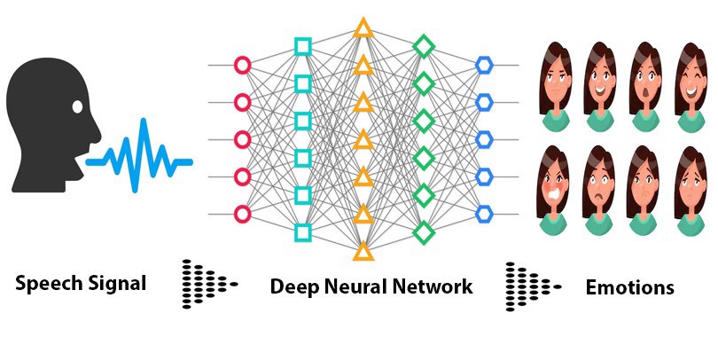

Speech Emotion Recognition Using Deep Learning

Introduction

The recognition of emotion in human speech is a widely researched topic, as there are many different applications that would directly benefit from this technology such as real time customer service as well as providing additional support for individuals with hearing impairments. With the ability to accurately decipher someone’s emotion based on how a sentence is spoken can vastly aid those who are deaf by providing additional social cues that may not be existent due to their condition. A real time classification of emotion throughout a conversation would also aid customer service of companies and provide further customer satisfaction by classifying the emotion of customers in real time.

Datasets

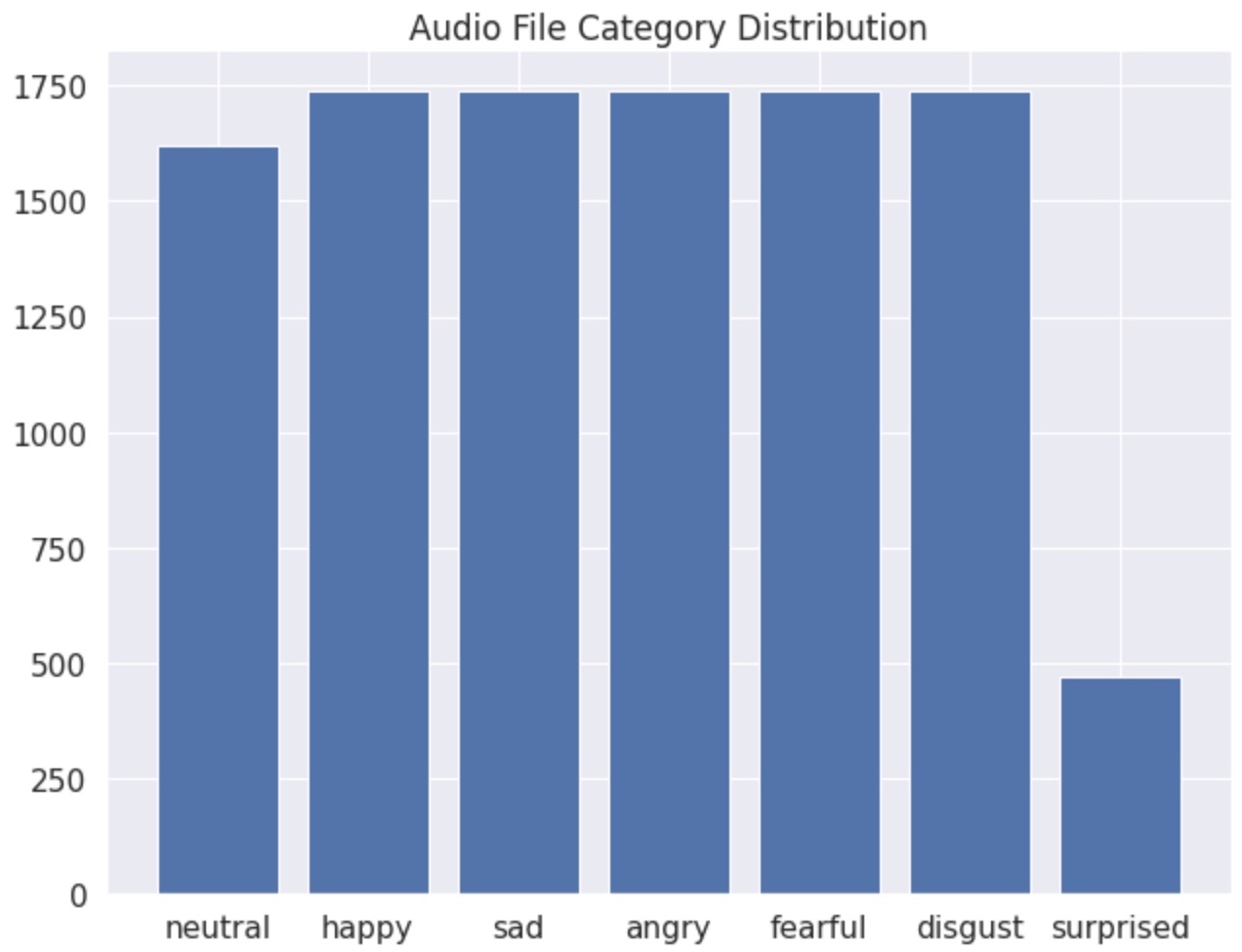
The datasets used in the creation of the models we created was an open source dataset collected from kaggle which can be viewed here. This dataset contains the following popular speech emotion datasets all in one: Crema, Ravdess, Savee, and Tess. This dataset contains audio files with labeled emotions in the filename. The labeled emotions vary from the 4 datasets, but as will be described in the methodology, only a certain number of emotions were kept in the final models outputted due to a variety of factors such as data constraints and dimensionality reduction in the modeling process. in total, there are 12,142 audio files all in english and saying a multitude of different sentences with different tones and emotions.

From Audio to Arrays

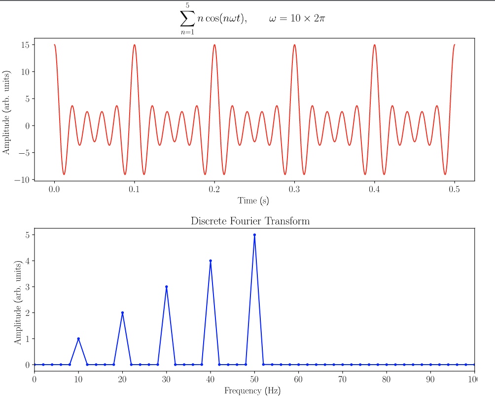
There are several audio processing methods avilable but for this study, we mainly focused on Mel Frequency Cepstral Coefficient (MFCC) and mel spectrograms. Audio data can be viewed as a signal with different frequencies with corresponding amplitudes propagating through time. A Fast Fourier transform (FFT)is a applied on a small time window of the signal to convert it from the time domain to a represenation in the frequency domain.

For MFCC’s, the log of the magnitude of the frequencies of the fourier transform are warped on a Mel Scale, followed by a inverse of a discrete continuous transform. The mel scale is a perceptual scale that maps frequencies to a percpetual scale of pitches judged to be in equal distance by listeners. The resulting transformation is a 2D array of the intensities of the mel coefficients over time.

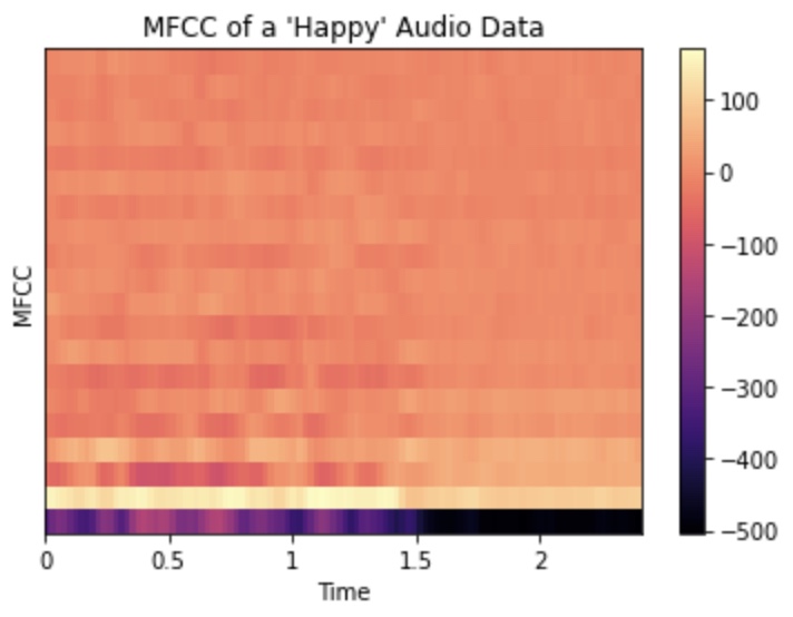
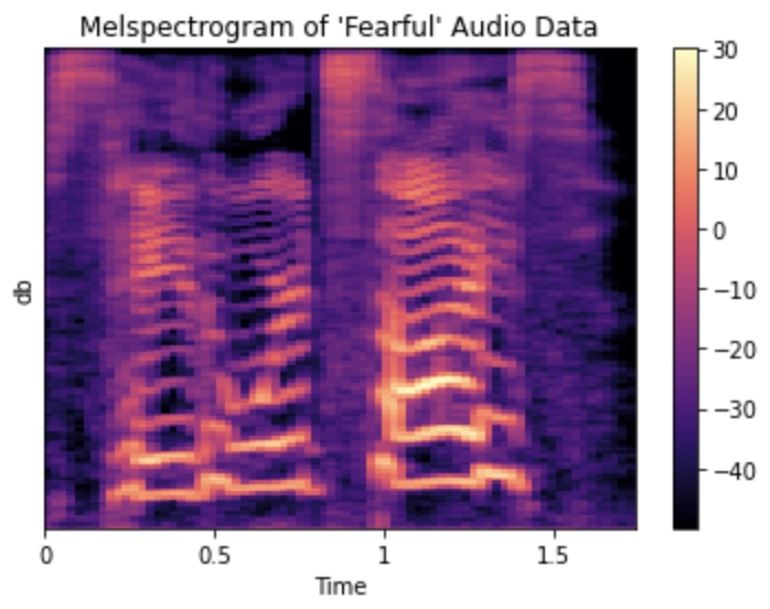
The mel spectrogram is similar to MFCC but wtih less mathemical operations. The spectrogram generated after the Fourier transform is converted into a mel scale. In this following figure, db units were used with 80db as the limit.

Methodology

Before modeling our data, we first needed to perform the ETL process as well as clean our data. The ETL process was straight forward, as all of our data was in a downloaded directory containing sub folders with all the audio files within each dataset. After downloading the dataset, we set out to create a pandas dataframe containing the path to the dataframe along with the features extracted from the audio file, and lastly the labeled emotion taken from the name of the audio file. In order to extract features from each audio file, we used the audio features that could be easily extracted from the librosa package. For the traditional machine learning models, we extracted the first 50 mel frequency cepstral coefficients (MFCCs), the first 50 mel spectogram values, the linear prediction coefficients in the 12th order, the root mean squared value for each frame, and the mean zero crossing value for the specified audio file. These features were then passed into the featurewiz method in order to programmatically select relevant features and drop highly correlated features. Featurewiz utilizes the XGBoost algorithm and correlation coefficients in order to extract the best “minimum optimal” features and drop highly correlated features .

While traditional ML methods require some extensive feature engineering, Neural Networks can learn the optimal features for the assigned task. Since the MFCCs and the mel spectrograms can be viewed as images, a CNN would be suitable for this classification problem. For the 1D Convolutional Neural Network, the preprocessed data used to train the traditional machine learning models was transformed into a 1D tensor. For the 2D Convolutional Neural Network, all 20 MFCC coefficients were extracted for the first 50 sec of the audio file to create a 2D array. The mel spectragram was also processed for each audio file utilizing the first 50 sec and first 20 Mel coefficients. The melspectgrams were transformed to a log decibel scale with a limit of 80 db and the sampling rate for every feature extraction was standardized at 22050. The two arrays were stacked to create a (2,20,50) tensor.

Traditional Machine Learning Models

For the traditional machine learning and deep learning models, we attempted to solve a multi-class classification problem around 4 different emotions: happy, sad, angry, and neutral. The models tested include random forests, support vector machines, and decision trees. The features that are considered most important by featurewiz and the XGBoost algorithms include melspectograms (especially around the 13th - 14th frame) the first few mfcc values, and the mean zero crossing value. This is expected, because as seen in past research, MFCC values and melspectogram values were also deemed important features in these studies as well. In order to evaluate the traditional machine learning models, we filtered our original dataset into these 4 emotions and then performed an 80/20 train test split where the testing data was not touched until the evaluation phase of the pipeline. After training, testing, and evaluating our models, we found that the random forest model performed best out of the traditional machine learning models, as seen in the results tab.

Neural Networks

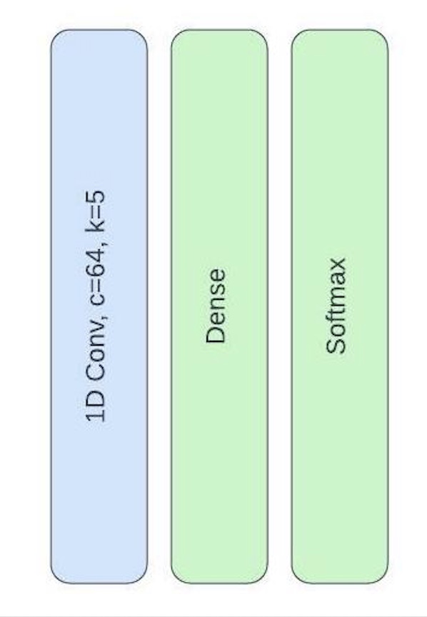
For the 1D CNN, The network contained a single convolutional layer (kernel size=5) followed by a ReLU activation layer and a dropout layer (p=0.5). The layer was then flattened followed by a dense layer and softmax regression.

For the 2D CNN, pytorch was utilized along with a CUDA GPU to speed up training. The network architecture involved two convolutional layers (stride=2, kernel size=(2,5)) followed by a (2,2) pooling layer. Another convolutional layer is added with the same parameters then a dense layer followed by softmax regression. A dropout layer was added (p=0.5) before every ReLu activation step which was added after each convolutional or dense layer. The model was trained at 20 epochs with a max learning rate (0.001), a negative log likelihood loss and ADAM as optimizer.

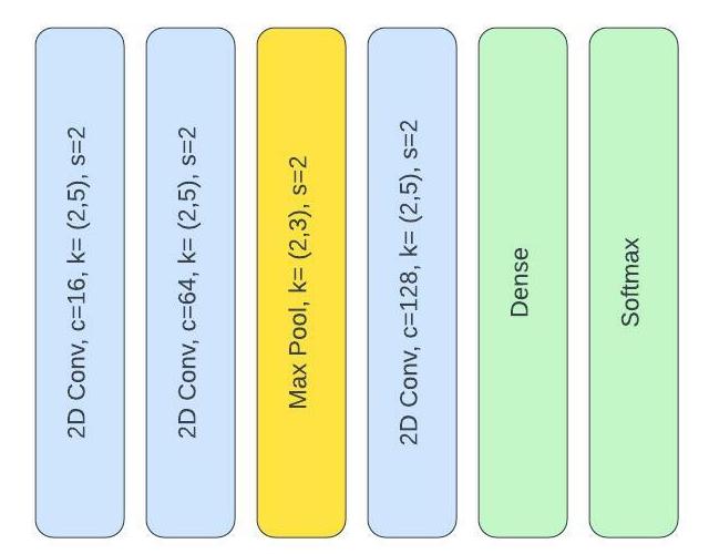
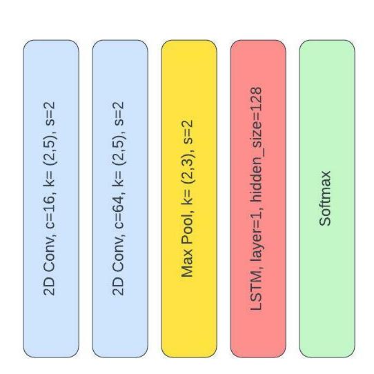
A third model was utilized using a CNN layer for feature extraction before a Long Short-Term Memory (LSTM) network. The feature extractor contained two convolutional layers and a max pool layer. The bidirectional LSTM has 128 hiddern layers with 1 layer size. The output was followed by a softmax layer. The model was trained at 100 epochs with cross entropy loss as the loss function and ADAM as optimizer.